Note: This post belongs to the blog-series ‘Understand SAP EWM’. The purpose of these series of blog-posts/videos is to explain the concepts of the core features of SAP EWM in a simple way. I want to focus on the basic understanding rather than the smallest details. For those of you who are a bit more experienced I will soon publish a blog/video about how to enhance the standard warehouse order creation rules.
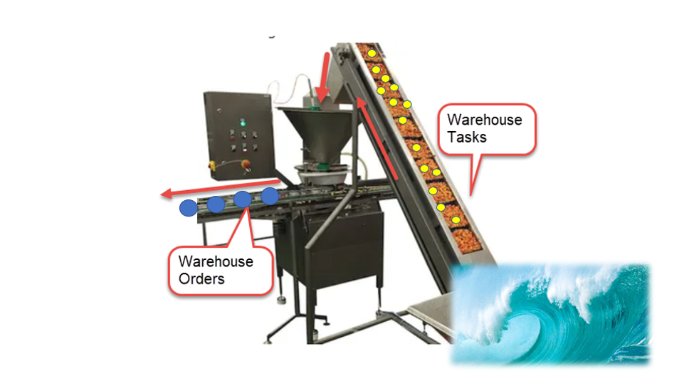
We start here by understanding that the WOCRs get warehouse tasks as an input and give warehouse orders as an output. WOCRs are being applied upon wave release respectively during other options (e.g. manual WT creation against an ODO) where we trigger the warehouse task creation.
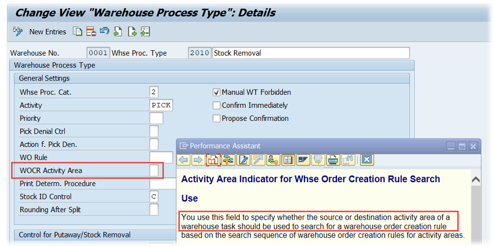
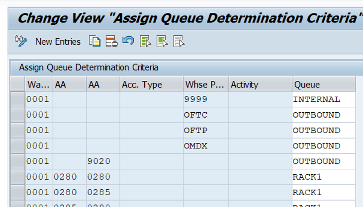
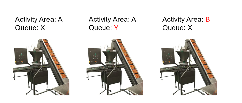
This happens separately for each combination of Activity Area and Queue. In other words – once created, the tasks are grouped by queue and activity area (the decision whether it is source or destination AA is based on the WOCR AA of the WPT). So a warehouse tasks with a different queue or a different activity area can never end up in the same warehouse order:
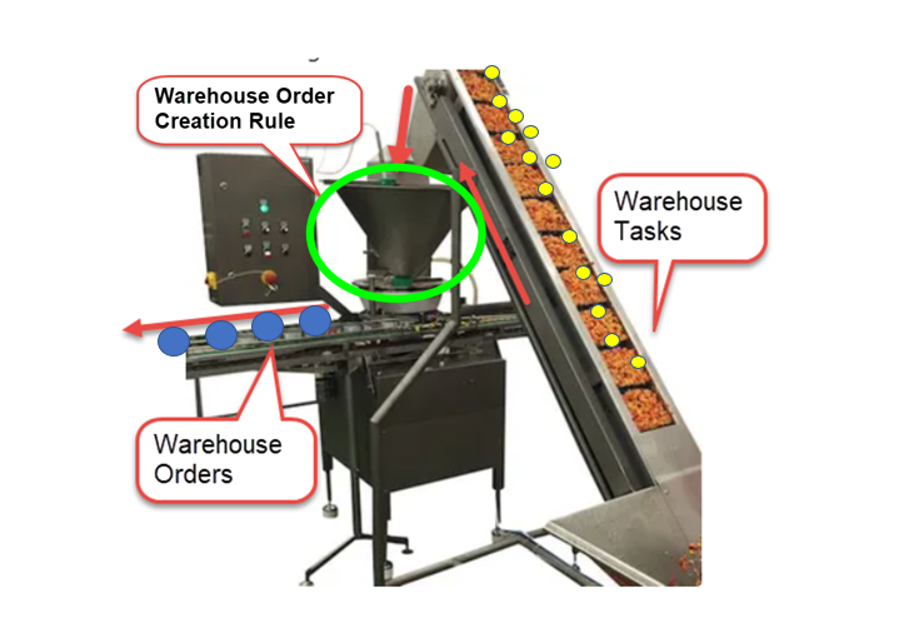
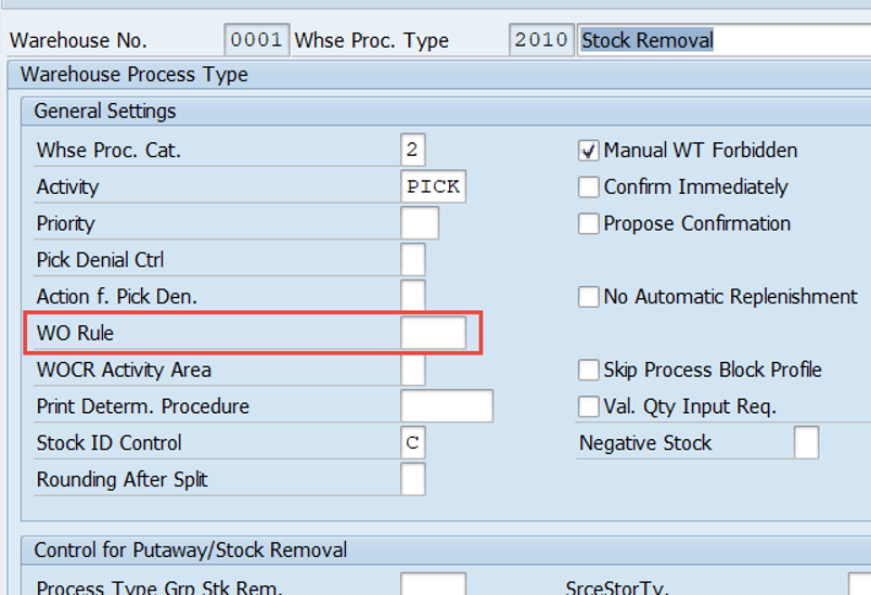
The first real WOCR-related step is the determination of the WOCR itself. This can be either pre-defined via the warehouse process type or based on the source/destination AA and the activity itself):
We will come to the determination as such later again. Let us here assume that we’ve found a WOCR which we want to apply now.
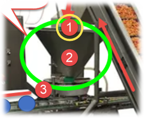
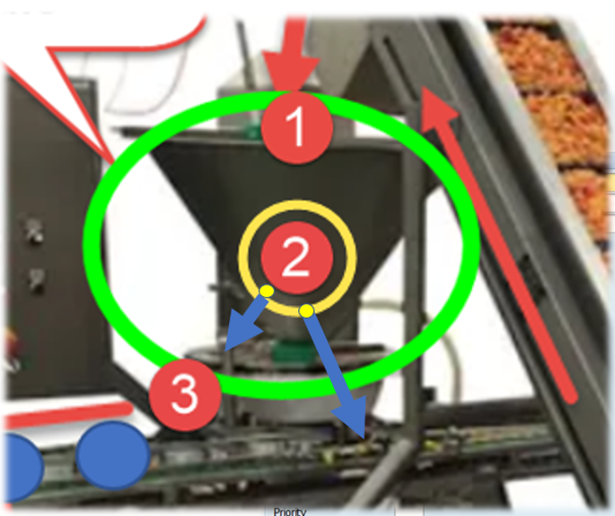
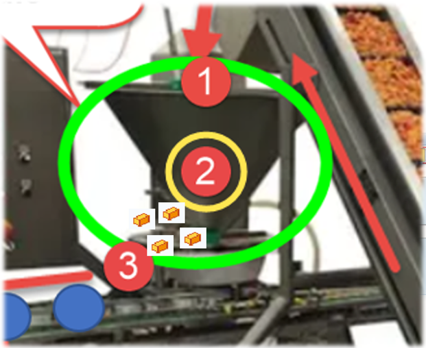
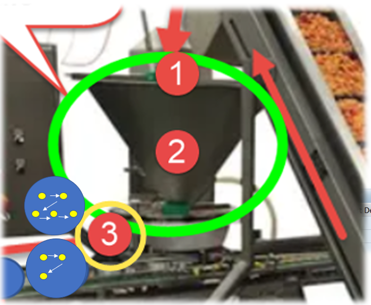
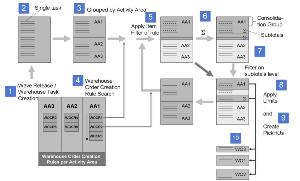
So what happened in this preparation phase (the (1) in the graphic below) so far? – We created the tasks – We grouped by AA and queue – We picked a WOCR for processing
The last step of the preparation (logically) is the inbound sorting from my point of view. During runtime this is actually happening after the item filter but the sequence between sorting and filtering doesn’t matter and I want to make it easy to undestand here:
What happens next can roughly be separated into another two areas (the 1st one we already covered): 2. Core 3. Closure
Let us proceed with the core logic:
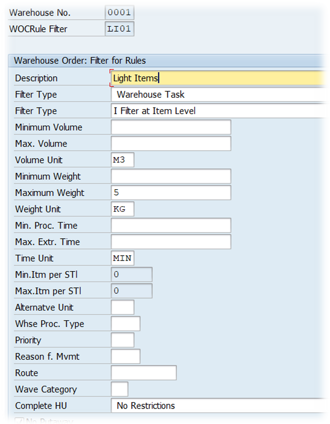
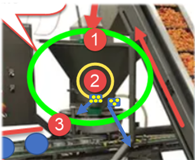
In the core area we we first apply filters on item level (e.g. filter out single tasks based on warehouse process type, wave template type or maximum weight/volume) before we apply filter on subtotal/CG levels (e.g. filter out complete consolidation groups (all tasks with the same group) with less than X WTs):
Subtotal filter:
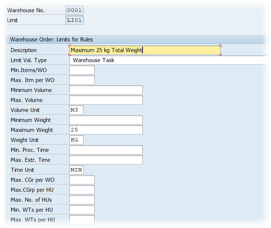
Next thing we do is to check limits on level of the warehouse order which is to be created. This could for example be the total weight/volume or the maximum number of WTs or Pick-HUs:
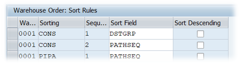
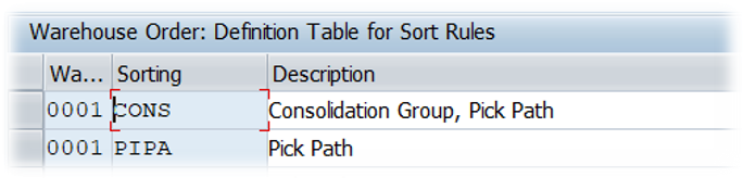
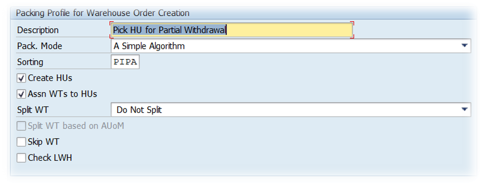
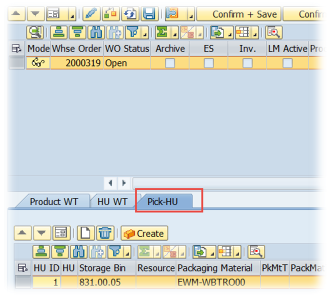
WTs which passed the filters and limits are sorted again and then tackled by the packing profile (where it is possible but not mandatory to create planned pick-HUs and assign the WTs to those HUs):
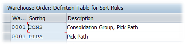
Now we come to what I call the ‘closure’. We sort the WTs again (3rd option now) but this time we are already within the WOs which have been created before:
That’s it!
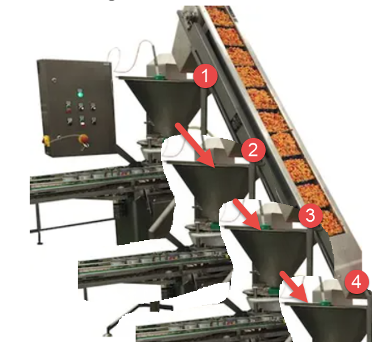
The warehouse orders are finally created. Not that complex at all isn’t it? Still the remaining question is what happens with those WTs which got sorted out? The answer is that we can have more than one of those ‘WOCR-Machines’. So once a WT got sortet out it will automatically be processed by the next WOCR with the same steps explained above for the first one:
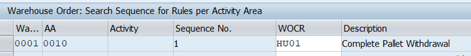
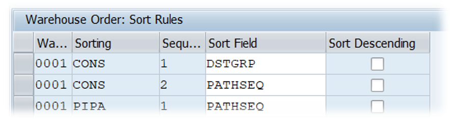
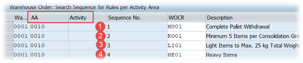
The sequence in which multiple WOCRs are being applied for a given warehouse tasks is defined in customizing – again based on AA and activity:
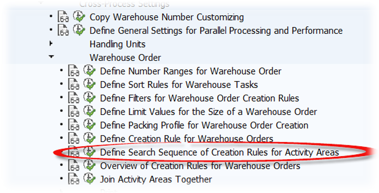
To sum it up –
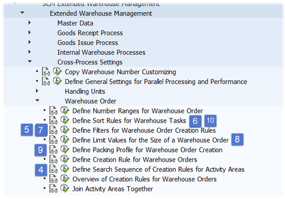
you’ll find a rough overview below showing the sequence of steps along with the customizing node:
I hope this blog post provides value to you and you could learn something. Please feel free to subscribe to my blog updates or my youtube channel in case you want to be notified about new posts!
We use cookies to ensure that we give you the best experience on our website. If you continue to use this site we will assume that you are happy with it.Ok